SEO PROJECT
One of my tasks as a marketing assistant was the search engine optimisation of the company’s website and blog and it wake my interest whether these tools that we use have a showable effect. To answer this question, writing my thesis at the university, through a review of the literature, I have selected the most widely used tools and then examined their impact on the chances of achieving a better ranking.
For the empirical study, 22 search terms were used to determine the effect of using the tools in the case of the top eight ranked pages. Since the ranking is on ordinal scale, I used ordinal logistic regression for the analysis.
More about search engine optimalization
We gather a lot of information through search engines, one of the biggest pieces of which is researching products and services before we buy. It is fair to say that nowadays the amount of information available online about a product group, brand or specific product exceeds the amount of information available offline.
Which information we come across in our search, out of the countless available, is decided by the search engines. As these tools influence the daily decisions of the masses, it is important to be aware of how they work.
Naturally, where there are a large number of potential consumers, marketing interfaces and solutions will inevitably emerge at some point. This is no different for search engines. Nowadays, on the one hand, several techniques are widely used by marketing professionals to move up in search results, and on the other, search engines have also emerged with paid services to enable companies that pay enough to secure a prominent position.
Search engines have been with us for more than twenty years. In that time, both the companies producing the content and the consumers searching for it have come a long way. As search engine optimisation technologies have become more sophisticated and more popular, the number of sites competing for top rankings has grown significantly. Since search engine optimisation is a zero-sum game, as competition increases, more and more are required to rank well. This perspective also gave rise to my research question: can the best-known techniques still work in 2022? To answer this question, I examined the extent to which the use of each technique influences the ability to achieve a better ranking for 22 keywords drawn from different topics.
Which SEO techniques did I examined?
To assess which tools are the most popular, I looked at the proportion of them mentioned in the literature. For this purpose, I have considered 20 studies from the last two decades.

Sources
An, S., & Jung, J. J. (2021): A heuristic approach on metadata recommendation for search engine optimization. Concurrency and Computation: Practice and Experience, 33(3), e5407.
Benczúr, Z. (2008): Keresőmarketing Google-organikus találati lista (Doctoral dissertation, BCE Gazdálkodástudományi Kar).
Dou, W., Lim, K. H., Su, C., Zhou, N., & Cui, N. (2010): Brand positioning strategy using search engine marketing. MIS quarterly, 261-279.
Evans, M. P. (2007): Analysing Google rankings through search engine optimization data. Internet research.
Gregurec, I., & Grd, P. (2012, September): Search Engine Optimization (SEO): Website analysis of selected faculties in Croatia. In Proceedings of Central European Conference on Information and Intelligent Systems (pp. 211-218).
Gunjan, V. K., Kumari, M., Kumar, A., & Rao, A. A. (2012): Search engine optimization with Google. International Journal of Computer Science Issues (IJCSI), 9(1), 206.
Khan, M. N. A., & Mahmood, A. (2018): A distinctive approach to obtain higher page rank through search engine optimization. Sādhanā, 43(3), 1-12.
Kovács, K. (2011): Organikus vagy szponzorált találatok: A keresőoptimalizálás összehasonlítása a fizetett hirdetésekkel (Doctoral dissertation, BCE Gazdálkodástudományi Kar).
Weideman, M., & Kritzinger, W. (2017): Parallel search engine optimisation and pay-per-click campaigns: A comparison of cost per acquisition. South African Journal of Information Management, 19(1), 1-13.
Leung, C. H., & Chan, W. T. (2021): A study on key elements for successful and effective search engine optimization. The International Journal of Technology, Knowledge, and Society.
Luh, C. J., Yang, S. A., & Huang, T. L. D. (2016): Estimating Google’s search engine ranking function from a search engine optimization perspective. Online Information Review.
Morauszki, T. (2015): A Google AdWords keresőhirdetés, mint marketingkommunikációs eszköz: Javaslatok a Google AdWords keresőhirdetés alkalmazására szakértői vélemények alapján (Doctoral dissertation, BCE Gazdálkodástudományi Kar).
Nagpal, M., & Petersen, J. A. (2020): Keyword selection strategies in search engine optimization: how relevant is relevance?. Journal of Retailing.
Palanisamy, R., & Liu, Y. (2018): User Search Satisfaction In Search Engine Optimization: An Empirical Analysis. Journal of Services Research, 18(2), 83-120.
Saberi, S., Saberi, G., & Mohd¹, M. (2013): What does the future of search engine optimization hold? International Journal of New Computer Architectures and their Applications (IJNCAA) 3(4): 132-138
Szabó, K. (2008): A keresőmarketing szerepe a Vichy Normaderm újrabevezetési kampányában (Doctoral dissertation, BCE-Gazdálkodástudományi Kar).
Sztankovics, G. V. (2020): Az online marketingeszközök lehetőségeinek vizsgálata és alkalmazása a mikro-, kis-és középvállalkozások működésében (Doctoral dissertation, BCE Gazdálkodástudományi Kar).
Ullah, A., Nawi, N. M., Sutoyo, E., Shazad, A., Khan, S. N., & Aamir, M. (2018): Search engine optimization algorithms for page ranking: comparative study. International Journal of Integrated Engineering, 10(6).
More about the mentioned techniques
Meta fields are parts of the source code of web pages that summarise the content of the page and are not necessarily visible to users. The algorithm looks at the code of web pages and pays attention to the content of these fields. One of the most important of these is the page title, which, in addition to this aspect, may also be important because it is one of the pieces of information that consumers encounter on the search engine results page (SERP). An attention-grabbing, relevant title can contribute to a higher number of clicks on a page link. Leun and Chan's (2019) research also shows that the use of parentheses and numbers can also be attention-grabbing for search engines, which can even lead to more clicks and higher rankings. Also, the dual role of the meta description is the same, as it is an important indicator for the algorithm as a meta field and can attract the interest of consumers on the search page. Another important field is the keyword (An - Jung, 2019), which, although typically not visible to visitors, can provide the search engine with information about the topic of the page.
About the database
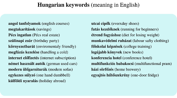
The data was collected in October 2022 using Google, the relevant sites and a marketing software called SERanking. The research identified 22 keywords that are diverse in terms of the industry.
SERanking estimates that there are approximately 1000 searches per month for the selected keywords.
As the first search page contains a different amount of advertising for each search term, the number of organic results will also vary. For the keywords I examined, there were between 7 and 10 pages on the first page, but as there were a total of 12 observations from the ninth and tenth rankings, I have excluded these from the analysis. In addition, 6 additional observations were removed from the database due to the lack of certain data, giving me a total of 170 observations to use in the research.
About the variables
The dependent variable is the ranking of the page in the search results, excluding ads.
The explanatory variables showed in the table below are selected from first table considering the number of mentions and the measurability.

Most of the variables give information whether certain parts of the page contain the keyword, so these are chategorichal variables. Besides these, with the help of SERanking, I collected the numerical value which gives information about the quality of the links pointing to the page and the estimated traffic.
The softver ranks the quality of the links pointing to a given page on a scale from one to onehundread, with a similar method of those used in part of Google’s algorithm, called PageRank. This means that both SERanking and PageRank pay attention to the numbers of the links pointing to the page, but they also evaluate the origin of the links. For example, a link from a page with big traffic, like a well-known news site worths more than a link from a less trustworthy page.
SERanking estimates the organic traffic based on how many keywords does the page rank for and how many searches there are for these keywords. This does not cover the whole traffic of a given page as visitors can also arrive from other channels like social media, but considering we don’t have the data about the page’s whole traffic I think the organic traffic is good to illustrate the difference in magnitude between the pages.
Descriptive statistics
CODE
#Descriptive statistics
View(SEO)
str(SEO)
summary (SEO)
#Changing the dummy variables to factors
SEO$rank <- factor (SEO$rank)
SEO$title <- factor (SEO$title)
SEO$URL <- factor (SEO$URL)
SEO$keyword <- factor (SEO$keyword)
SEO$picture <- factor (SEO$picture)
SEO$H16 <- factor (SEO$H16)
SEO$sitemap <- factor (SEO$sitemap)
SEO$description <- factor(SEO$description)
SEO$social <- factor(SEO$social)
psych::describe(SEO[,c(3,11)])
lapply(SEO[, c("title",
"URL",
"keyword",
"description",
"picture",
"H16",
"sitemap")], table)
ftable(xtabs(~ rank + title, data = SEO))
ftable(xtabs(~ rank + URL, data = SEO))
ftable(xtabs(~ rank + keyword, data = SEO))
ftable(xtabs(~ rank + description, data = SEO))
ftable(xtabs(~ rank + picture, data = SEO))
ftable(xtabs(~ rank + H16, data = SEO))
ftable(xtabs(~ rank + sitemap, data = SEO))
#Visulizing the data
theme_set(theme_light(base_size = 8))
kat<-inspect_cat(SEO[,c(2,4,5,6,7,8,9,10)])
kat
show_plot(kat, text_labels = TRUE)
plot2.1 <- ggplot(SEO)+ aes(x = title) +
geom_bar(fill="cadetblue2")
plot2.2 <- ggplot(SEO)+ aes(x = keyword) +
geom_bar(fill="cadetblue2")
plot2.3 <- ggplot(SEO)+ aes(x = URL) +
geom_bar(fill="cadetblue2")
plot2.4 <- ggplot(SEO)+ aes(x = description) +
geom_bar(fill="cadetblue2")
plot2.5 <- ggplot(SEO)+ aes(x = picture) +
geom_bar(fill="cadetblue2")
plot2.6 <- ggplot(SEO)+ aes(x = H16) +
geom_bar(fill="cadetblue2")
plot2.7 <- ggplot(SEO)+ aes(x = sitemap) +
geom_bar(fill="cadetblue2")
plot2.8 <- ggplot(SEO)+ aes(x = social) +
geom_bar(fill="cadetblue2")
grid.arrange(plot2.1, plot2.2, plot2.3, plot2.4,
plot2.5, plot2.6, plot2.7, plot2.8, ncol=3)
plot1 <- ggplot (data = SEO) +
geom_boxplot (aes(x=backlink), fill="cadetblue2")
plot2 <- ggplot (data = SEO) +
geom_boxplot (aes(x=traffic), fill="cadetblue2")
grid.arrange(plot1, plot2, ncol=2)
#There are clearly visible outliers which I exclude from the dataset in order to make the analysis easier
SEO <- SEO[-c(9,10,36,37,61), ]
plot1 <- ggplot (data = SEO) +
geom_boxplot (aes(x=backlink), fill="cadetblue2")
plot2 <- ggplot (data = SEO) +
geom_boxplot (aes(x=traffic), fill="cadetblue2")
grid.arrange(plot1, plot2, ncol=2)
#The distribution is still left-skewed, so I take the logarithm of these variables
ggplot (data = SEO) +
geom_histogram (aes(x=log(traffic)), fill="cadetblue2")
ggplot (data = SEO) +
geom_histogram (aes(x=log(backlink)), fill="cadetblue2")
SEO$logbacklink <- log(SEO$backlink)
boxplot_1<- qplot(x = rank, y = logbacklink, data = SEO, geom = "boxplot", fill = rank)
boxplot_1 + xlab("rank") + ylab("log(backlink)")
SEO$logtraffic <- log(SEO$traffic)
boxplot_1<- qplot(x = rank, y = logtraffic, data = SEO, geom = "boxplot", fill = rank)
boxplot_1 + xlab("rank") + ylab("log(traffic)")
In case of the numeric variables, I observed the outliers in my database with the help of boxplots. Both the traffic and a backlink variable have some outliers. Although it doesn’t necessarily comes from an error of data collection, I excluded the three outliers visible in the plot bellow and the four more from the analysis.

The of the variables is still left skewed based on the plots bellow, which is also supported by the fact, that the average is below the median and skewness indicator is positive. For this reason, I took the logarithm of these two variables while analysing the data.

From the categorical variables the keyword was used most time (102) in the title. This was followed by mentioning the keywords in the headings with 94 observation and putting it to the URL and the meta description with 78 and 77 observations. Among the meta keywords the searched keyword was mentioned by less than the quarter of the pages. Based on this we can say that the techniques mentioned more frequently by the literature were applied as well more often in the practice.

About the variable representing the social media we can say that almost 75% of the pages are present at least 3 social media sites and there is only three brand that have no social media sites at all.
The frequency of the outcome variable is quite similar due to the sampling method.
Analysing bivariate relationships
CODE
#Chi square test 0,99
test1 <- chisq.test(table(SEO$rank, SEO$title))
test2 <- chisq.test(table(SEO$rank, SEO$URL))
test3 <- chisq.test(table(SEO$rank, SEO$keyword))
test4 <- chisq.test(table(SEO$rank, SEO$description))
test5 <- chisq.test(table(SEO$rank, SEO$picture))
test6 <- chisq.test(table(SEO$rank, SEO$H16))
test7 <- chisq.test(table(SEO$rank, SEO$sitemap))
test8 <- chisq.test(table(SEO$rank, SEO$social))
test1
test2
test3
test4
test5
test6
test7
test8
cramerV(ftable(xtabs(~ rank + title, data = SEO)))
cramerV(ftable(xtabs(~ rank + URL, data = SEO)))
cramerV(ftable(xtabs(~ rank + keyword, data = SEO)))
cramerV(ftable(xtabs(~ rank + description, data = SEO)))
cramerV(ftable(xtabs(~ rank + picture, data = SEO)))
cramerV(ftable(xtabs(~ rank + H16, data = SEO)))
cramerV(ftable(xtabs(~ rank + sitemap, data = SEO)))
After the descriptive statistic, I examined the bivariate relationship between the outcome variable and the categorical variables pairwise. Given the ordinality of the variables I used the Chi square test to decide, whether the outcome variable is independent from the explanatory variables. With 5 percent significance level I reject the hypothesis, that the categorical variables are independent from the outcome variable.

After this I examined the strength of these relationships with the help of the Cramer measurement. This number was below or close to 0,2 in the case of every categorical variable, which mean only a weak relationship.
Selection of the model
CODE
#First model with all the variables
mod <- polr (rank ~ title + log(backlink) + URL + keyword + description + picture + H16 + sitemap + social + log(traffic), data= SEO, Hess = T)
summary (mod)
ctable <- coef(summary(mod))
p <- pnorm(abs(ctable[, "t value"]), lower.tail = FALSE) * 2
OR <- exp(coef(mod))
ctable <- cbind(ctable, "p value" = p, "OR" = OR)
stargazer::stargazer(ctable, type="text", digits=4, out = "ctable.html")
#Second model with the significant variables of the previous model
mod2 <- polr (rank ~ social + sitemap + log(traffic), data= SEO, Hess = T)
summary(mod2)
ctable2 <- coef(summary(mod2))
p2 <- pnorm(abs(ctable[, "t value"]), lower.tail = FALSE) * 2
ctable2 <- cbind(ctable, "p value" = p2)
ctable2
#Comparing the two models
PseudoR2(mod, "McFadden")
PseudoR2(mod2, "McFadden")
BIC(mod)
BIC(mod2)
AIC(mod)
AIC(mod2)
As the first step I included all variables mentioned in the first sheet, but with 5 percent significance level only the traffic and the social media variables were significant, and the sitemap variable fell also close to the border value.
For the next model therefore I used these three variables. For compering the two models I used the Schwartz, Akaike and McFadden-R2 indexes. While the Schwartz index improved with using the second model, based on the other two measurment it is better to choose the first one. In the case of the McFadden-R2 we can mention, that although some decay was expected as the measurements based on the discipline of the R2 usually decline with the declining of the number of explanatory variables, but in this case almost one third of the explanatory force was lost.

Results
Because of the results described in the previous part I decided to keep all of the explanatory variables in my model. The results of my model can be seen in the next table.
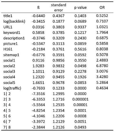
The odd ratio shows the relative probability of belonging to a group compered to any other lower ranking group.
In the case of traffic for example 1 percent incresement with everything else staying the same increases the probability of belonging to a higher category with 46 percent. Based on the p values the traffic seems the most significant variable, which paired with a higher OR than expected implies an important conclusion. As the traffic and the ranking are in a reciprocal relationship with each other, we can guess that keeping a good position is easier than reaching one.
By the other significant value, the social media I expected monotone decrisment from the first to the fifth level, so that the more social media sites are a page present, the higher the probability is for reaching a better position. In contrast, my results showed the highest value in the fifth and second category.
The other variables are not proven significant, so I didn’t analyse their odds ratio. Based on the p value the increasing of the variables (which in the case of the categorical variables means turning to 1 from 0) doesn’t effect the reaching of a better position.
My results differ from the findings of previous research on several points. Nagpal and Petersen's (2020) study looked at rankings as a function of online authority, content relevance, search progression and degree of competition. In their model, online authority was included as a combination of page authority and domain authority, which gives a reason to compare the results with the backlink variable in my model, which is also related to the value of page authority. Their results show that, unlike mine, the variable is significant at the five percent significance level. The difference, beyond the fact that the indicator in their case contains information not only about the URL but also about the whole website, may also stem from the fact that their variable is relative, with values relative to competitors. I did not consider this kind of relativisation to be important due to the similar search volume between the variables considered in my research. In addition, the two researchers considered the first fifty results, which may also cause reach, due to the claim described earlier that the algorithm may not necessarily use the same ranking among the top search results as it does on either of the other pages of the search result.
Also for comparison, the Content Relevance variable from Nagpal and Petersen's (2020) research, for which the title of the pages was examined, provides a comparison. Their observation is significantly different from my result for the variable cim, which is significant at the 5% significance level. In the case of my database, this variable already showed the weakest relationship with the outcome variable when the Cramer indicators were calculated and was not found to be significant in the model. This discrepancy may also be due to the difference in data collection, as the two researchers also used a more sophisticated method to investigate the semantic relationship between the keyword and the other terms in the title.
Also in contrast to my results is the research of An and Jung (2019), who also found that the optimization of meta fields can improve the ranking of a URL when designing an appropriate keyword targeting method. In contrast, the title, meta description, and meta keyword were not found to be significant in the model I built.
In terms of the frequency of use of these tools, however, my finding, mentioned in the descriptive statistics section, is in line with the work of Leun and Chan (2021), who also found that the most frequent of the on-page tools is the mention of a keyword in the title, followed by a small lag in the frequency of mentioning it in the meta description, and the two indicators are followed by a much smaller proportion of mentioning the keyword in the meta keyword.
Comparing my results with the literature
The limitations of my model
CODE
#Multicollienarity test
car::vif(mod2)
#Testing the assumption of proportionality
sf <- function(y) {
c('Y>=1' = qlogis(mean(y >= 1)),
'Y>=2' = qlogis(mean(y >= 2)),
'Y>=3' = qlogis(mean(y >= 3)),
'Y>=4' = qlogis(mean(y >= 4)),
'Y>=5' = qlogis(mean(y >= 5)),
'Y>=6' = qlogis(mean(y >= 6)),
'Y>=7' = qlogis(mean(y >= 7)),
'Y>=8' = qlogis(mean(y >= 8))
)
}
s <- with(SEO, summary(as.numeric(rank) ~ social + sitemap + traffic, fun=sf))
s[, 9] <- s[, 9] - s[, 8]
s[, 8] <- s[, 8] - s[, 7]
s[, 7] <- s[, 7] - s[, 6]
s[, 6] <- s[, 6] - s[, 5]
s[, 5] <- s[, 5] - s[, 4]
s[, 4] <- s[, 4] - s[, 3]
s[, 3] <- s[, 3] - s[, 3]
plot(s, which=1:9, pch=1:9, xlab='logit', main=' ', xlim=range(s[,3:9]))
The fact that my results contradict the findings of previous research, which may be due to, among other things, the different ways of defining the variables, raises the question of the correct metric for measuring each variable. Although the literature on search engine optimization has grown with a significant number of studies over the years, there is no generally accepted answer to the question of what is the appropriate method to measure the effectiveness of each technique. This may also be due to the lack of information on the metrics used by Google's search engine to evaluate a page. A good example is that while in my research I measured the relevance of the title by the presence of the keyword only, other research has taken into account the relative keyword density or even the semantic relationship of the terms contained in the title to the keyword. We do not know exactly which of these is used by the search engine, but with the accelerating development of technology, it is possible that even these involve a much more complex, multi-layered analysis, even for a field such as a title.
A further limitation of my model is the assumptions required to apply ordinal logistic regression. The lack of adequate sample size and multicollinearity in the model is present, however, I rejected the proportionality assumption by performing the graphical test suggested by Harell (2001). Thus, it is not true for the model that the relationship is the same for any pairwise comparison of the ranking categories, and the applicability of the logistic regression model is questionable.
Nevertheless, due to the sampling, my results are only applicable to the Google search engine and within that to the results of the first search page. The Hungarian search terms were part of my research, which also narrows down the general scope of my research, but I considered this narrowing down important because it gave me an idea of the frequency of use of the techniques by Hungarian sites, which I could not find any examples of in the previous literature. In addition, the results of the research may quickly become outdated due to the continuous updates of Google's search engine, as a change can then fundamentally change the way a site appears in search results.